1. DC Optimal Power Flow
Module 1 consists of the DC Optimal Power Flow and its mathematical model
- 1a is the Excel program Input and Output
- 1b is a guide leaflet for 1a
- 1c is the excel file which can be downloaded and used for experimentation and other purposes.
Introduction –
DC Optimal Power Flow – 3 Bus configuration
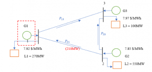
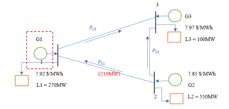
A 3-bus network is presented above. Note that there are three generators over bus 1, 2 and 3. The marginal cost of generator 1, 2 and 3 is $7.92/MWh (when it is built), $7.85/MWh and $7.97/MWh, respectively. The physical transmission limit of transmission line P12 is 210MW. The demand load at bus 1 is 270 MW, bus 2 is 550 MW and bus 3 is 100 MW, and the total demand load is 850 MW.
We consider two cases for this particular problem. In the first case, only two generators are being used by the whole network, i.e., and . The total demand is met by these two generators only. In the second case, we add a generator at node 1. Now, the total demand can be met by all the three generators. We will see in the following modules how adding a generator to node 1 in this network is beneficial in various ways.
Mathematical formulation for DCOPF model
1a. Excel Program Input/Output
Module 1a shows the excel program input values and output solution. Excel solver is used for this particular model. Since the objective function is linear, we can choose ‘Simplex LP’ or ‘GRG Nonlinear’ as the solver methodology.
The following diagrams are of both the cases that were mentioned in module 1. Case 1 is with only 2 generators at node 2 and 3. Case 2 is with 3 generators at all the nodes.
Case 1 – 2 generators
Input –
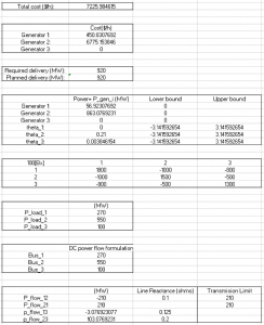
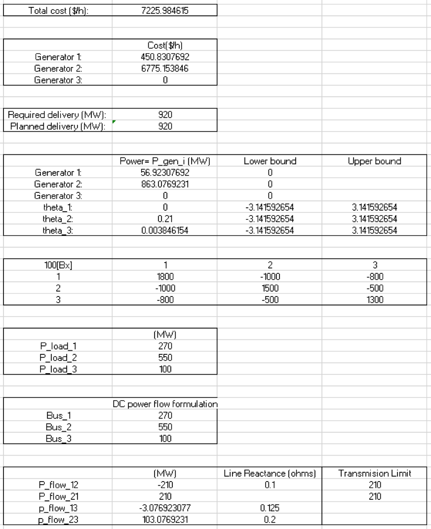
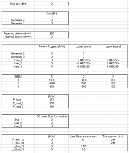 Output –
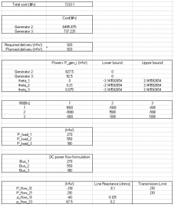 Case 2 – 3 generators
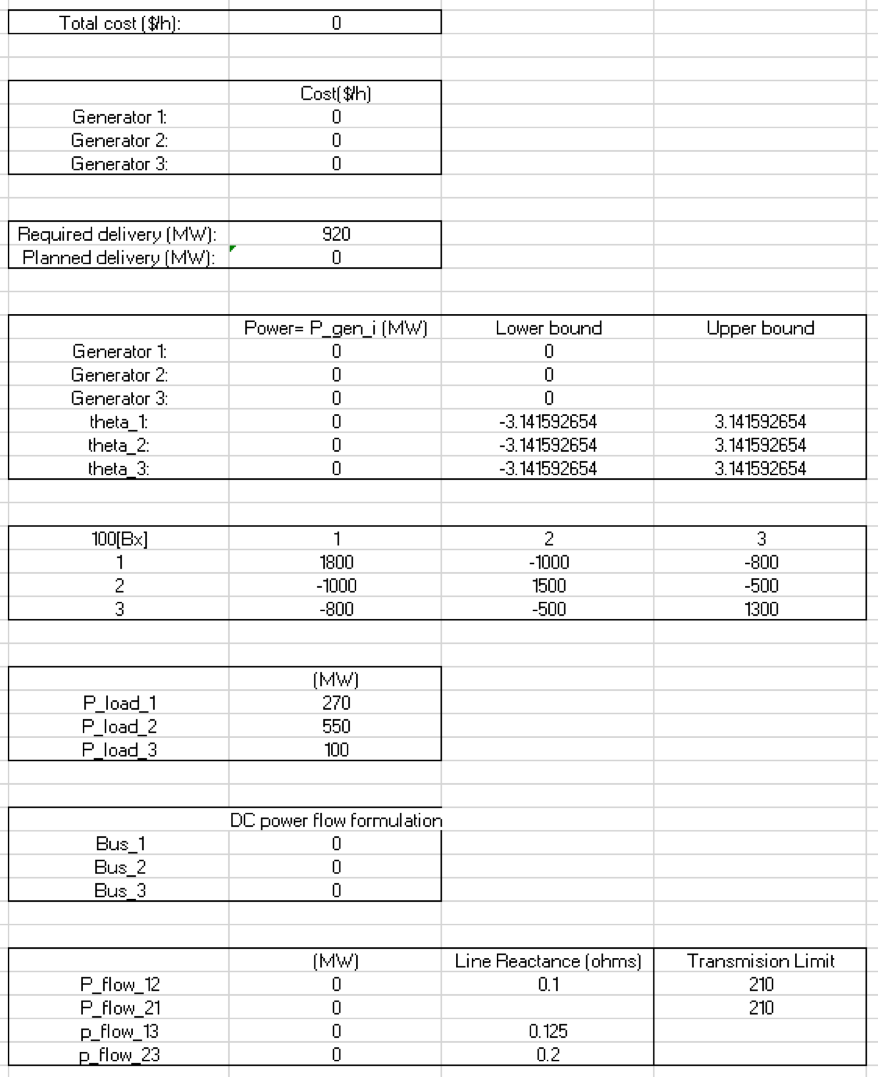
Input –
Case 2 – 3 generators
Input –
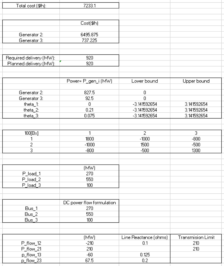
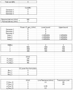 Output –
 Note – The total production cost decreases when we add generator at node 1 because the marginal cost of this generator is lower than G3 and the total demand is met by a combination of G2 and G1.
1b. Guide for Excel solver
Input for Excel Solver
Step 1 –
Note – The total production cost decreases when we add generator at node 1 because the marginal cost of this generator is lower than G3 and the total demand is met by a combination of G2 and G1.
1b. Guide for Excel solver
Input for Excel Solver
Step 1 –
Write down the variables in one column and values in the next column. Let the values be 0 initially. Similarly input the values of
Pload which are already given.
Step 2 –
Write the objective function which is to minimize the cost. The objective function is the total cost cell in the excel file.
Step 3 –
The constraints are already included the excel sheet. The lower bound and upper bound for theta should be kept as -3.14 to 3.14 radians. The lower bound of generation capacity is 0 and there is no upper bound given. The susceptance matrix has all the values needed for power flow calculations. The power flow limit in line 1-2 is also included with respective reactance.
Running Excel solver
Select Data (from top bar) => Solver. (Top right corner)
Step 1 – Set Objective – Select the cell where objective function has been written down.
Step 2 – To: Min
Step 3 – By changing variable cells: Select the whole column containing values of the variables p1, p2, p3,
θ1, θ2 and
θ3
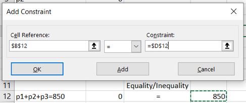
Step 4 – Subject to constraints: select ‘Add’
For Cell reference select the constraint equation cell, select appropriate equality/inequality sign, for Constraint select the cell with constraint value.
 Step 5
 – Do not select the option –
Make unconstrained variables non-negative
Step 6 – Select a solving method = GRG nonlinear or Simplex LP depending upon the objective function
Step 7 – Select ‘
Solve’
1c. Download Excel for experimentation and other purposes
Next module
 A 3-bus network is presented above. Note that there are three generators over bus 1, 2 and 3. The marginal cost of generator 1, 2 and 3 is $7.92/MWh (when it is built), $7.85/MWh and $7.97/MWh, respectively. The physical transmission limit of transmission line P12 is 210MW. The demand load at bus 1 is 270 MW, bus 2 is 550 MW and bus 3 is 100 MW, and the total demand load is 850 MW.
We consider two cases for this particular problem. In the first case, only two generators are being used by the whole network, i.e., and . The total demand is met by these two generators only. In the second case, we add a generator at node 1. Now, the total demand can be met by all the three generators. We will see in the following modules how adding a generator to node 1 in this network is beneficial in various ways.
Mathematical formulation for DCOPF model
1a. Excel Program Input/Output
Module 1a shows the excel program input values and output solution. Excel solver is used for this particular model. Since the objective function is linear, we can choose ‘Simplex LP’ or ‘GRG Nonlinear’ as the solver methodology.
The following diagrams are of both the cases that were mentioned in module 1. Case 1 is with only 2 generators at node 2 and 3. Case 2 is with 3 generators at all the nodes.
Case 1 – 2 generators
Input –
A 3-bus network is presented above. Note that there are three generators over bus 1, 2 and 3. The marginal cost of generator 1, 2 and 3 is $7.92/MWh (when it is built), $7.85/MWh and $7.97/MWh, respectively. The physical transmission limit of transmission line P12 is 210MW. The demand load at bus 1 is 270 MW, bus 2 is 550 MW and bus 3 is 100 MW, and the total demand load is 850 MW.
We consider two cases for this particular problem. In the first case, only two generators are being used by the whole network, i.e., and . The total demand is met by these two generators only. In the second case, we add a generator at node 1. Now, the total demand can be met by all the three generators. We will see in the following modules how adding a generator to node 1 in this network is beneficial in various ways.
Mathematical formulation for DCOPF model
1a. Excel Program Input/Output
Module 1a shows the excel program input values and output solution. Excel solver is used for this particular model. Since the objective function is linear, we can choose ‘Simplex LP’ or ‘GRG Nonlinear’ as the solver methodology.
The following diagrams are of both the cases that were mentioned in module 1. Case 1 is with only 2 generators at node 2 and 3. Case 2 is with 3 generators at all the nodes.
Case 1 – 2 generators
Input –
 Output –
 Case 2 – 3 generators
Input –
Case 2 – 3 generators
Input –
 Output –
 Note – The total production cost decreases when we add generator at node 1 because the marginal cost of this generator is lower than G3 and the total demand is met by a combination of G2 and G1.
1b. Guide for Excel solver
Input for Excel Solver
Step 1 –
Write down the variables in one column and values in the next column. Let the values be 0 initially. Similarly input the values of Pload which are already given.
Step 2 –
Write the objective function which is to minimize the cost. The objective function is the total cost cell in the excel file.
Step 3 –
The constraints are already included the excel sheet. The lower bound and upper bound for theta should be kept as -3.14 to 3.14 radians. The lower bound of generation capacity is 0 and there is no upper bound given. The susceptance matrix has all the values needed for power flow calculations. The power flow limit in line 1-2 is also included with respective reactance.
Running Excel solver
Select Data (from top bar) => Solver. (Top right corner)
Step 1 – Set Objective – Select the cell where objective function has been written down.
Step 2 – To: Min
Step 3 – By changing variable cells: Select the whole column containing values of the variables p1, p2, p3, θ1, θ2 and θ3
Step 4 – Subject to constraints: select ‘Add’
For Cell reference select the constraint equation cell, select appropriate equality/inequality sign, for Constraint select the cell with constraint value.
Note – The total production cost decreases when we add generator at node 1 because the marginal cost of this generator is lower than G3 and the total demand is met by a combination of G2 and G1.
1b. Guide for Excel solver
Input for Excel Solver
Step 1 –
Write down the variables in one column and values in the next column. Let the values be 0 initially. Similarly input the values of Pload which are already given.
Step 2 –
Write the objective function which is to minimize the cost. The objective function is the total cost cell in the excel file.
Step 3 –
The constraints are already included the excel sheet. The lower bound and upper bound for theta should be kept as -3.14 to 3.14 radians. The lower bound of generation capacity is 0 and there is no upper bound given. The susceptance matrix has all the values needed for power flow calculations. The power flow limit in line 1-2 is also included with respective reactance.
Running Excel solver
Select Data (from top bar) => Solver. (Top right corner)
Step 1 – Set Objective – Select the cell where objective function has been written down.
Step 2 – To: Min
Step 3 – By changing variable cells: Select the whole column containing values of the variables p1, p2, p3, θ1, θ2 and θ3
Step 4 – Subject to constraints: select ‘Add’
For Cell reference select the constraint equation cell, select appropriate equality/inequality sign, for Constraint select the cell with constraint value.
 Step 5 – Do not select the option – Make unconstrained variables non-negative
Step 6 – Select a solving method = GRG nonlinear or Simplex LP depending upon the objective function
Step 7 – Select ‘Solve’
1c. Download Excel for experimentation and other purposes
Step 5 – Do not select the option – Make unconstrained variables non-negative
Step 6 – Select a solving method = GRG nonlinear or Simplex LP depending upon the objective function
Step 7 – Select ‘Solve’
1c. Download Excel for experimentation and other purposes